Probability

This blog is a review of probability information.

• Probability Distributions
• Conditional Probability and Bayes Theorem
• Estimation: ML, MAP
• From condition probability to Bayesian Networks
• Example: Naive Bayes Model
• Example: Bayesian Tracking, Temporal Model and the Plate Model
• From Directed Model to Undirected Model
• Exact Inference
• Message Passing and Belief Propagation

Probability Distributions

• For a variable x, if it satisfies a distribution p(x), we can write as $x\sim p(x)$. The probability that x appears as a particular value $x_0$ is $p(x_0)$.
• A joint probability distribution for several variables is $p(x_1, x_2, …)$
• Several conditions of probability distributions:
  • Marginalization: $\int p(x) dx = 1$ (if x is continuous) and $\sum p(x) = 1$ (if x is discrete). The total probability is 1.
  • Marginalization for joint probability distributions: $\int p(x,y) dy = p(x)$
  • Factorization: $p(x,y)=p(x)p(y)$ if and only if x and y are independent
• Many people write probabiltiy distibutions as functions. $f_{x}(x_0)$, $p(x_0)$, and $p(x=x_0)$ are the same thing.

Conditional Probability and Bayes Theorem

• The probability of x given y: $p(x|y)=\frac{p(x,y)}{p(y)}$
• Bayes Theorem: $p(x|y)=\frac{p(y|x)p(x)}{p(y)}$
• If we interpret x as the variable, y as the observation, then $p(x)$ is “prior belief”, $p(y|x)$ is the likelihood, $p(y)=\sum_x p(y|x)p(x)$ is the nomalization constant, and $p(x|y)$ is the “a posterior” (“afterwards”) distribution. This idea is generalized in the Bayesian tracking, where the a posterior belief is updated every time when a new observation comes in.

Estimation: MLE, MAP

• Now that we have the probability distribution $p(\mathbf{x};\theta)$ where x is data and $\theta$ is (unknown) parameter.
• Define likelihood (function of $\theta$): $L(\theta; \mathbf{x})=p(\mathbf{x}|\theta)$ as the probability of getting such data given the $\theta$.
• Maximizing the likelihood function results in the Maximum Likelihood Estimation (MLE): $\theta^{MLE}=argmax_{\theta}p(x|\theta)$.
• Define the a posteriori probability as $p(\theta | x)$, which is the probability of $\theta$ given data x.
• Then the “maximum a posteriori probability” $\theta^{MAP}=argmax_{\theta} p(\theta|x)$ is the $\theta$ that results in a maximum a posteriori probability.
• Note that MAP can be calculated using MLE. $\theta^{MAP}=argmax_{\theta} p(\theta|x)=argmax_{\theta} \frac{p(x|\theta)p(\theta)}{p(x)}$ $$=argmax_{\theta} \frac{p(x|\theta)p(\theta)}{\sum_{\theta} p(x|\theta)p(\theta)}=argmax_{\theta}p(x|\theta)g(\theta)$$
• So when $g(\theta)$ is constant, MAP is the same as MLE.

From Condition Probability to Bayesian Network

• We have seen that random variables can interact with each other, as described by the dependencies.
• Using graphical model to represent the dependencies between variables is an intuitive way.
• Use nodes to represent random variables, and edges to represent dependency. $x \rightarrow y$ means the random variable x depends on y.
• To decide a joint distribution, we need a condition probability distribution for each node. For example, the joint probability distribution corresponding to the graph $x \rightarrow y$ can be written as $$f_{x,y}(x,y)=f_y(y)f_{x|y}(x|y)$$
• Such type of graph is called Bayesian Network (BN).
• Bayesian Network is one of the two most common Probabilistic Graphics Models (PGM). The other type of PGM is Markov Random Fields (MRF), where the graphs are undirected.
• The “model” in PGM refers to the machine learning models.
• There are at least two obvious benefits of using PGM. First, it provides a clear visualization of conditional dependence of variables. Dependencies, or inferences, of variables can flow within a Bayesian Network according to some rules (Bayes Ball or d-separation). Second, it provides a rich language and framework to describe machine learning algorithms.
• Two variables are said to be d-separated if dependency cannot flow from one to the other. There are four types of junctions:
  (1) $A\rightarrow S \rightarrow B$. When S is unobserved, dependency can flow from A to B. When S is observed, it can not.
  (2) $A \leftarrow S \leftarrow B$. Same as (1).
  (3) $A \leftarrow S \rightarrow B$. Same as (1).
  (4) $A \rightarrow S \leftarrow B$. “V-structure”. When S or any of successors of is observed, dependency can flow from A to B. It cannot otherwise. Why is this case different? Consider the example where A is “cleverness”, S is “score”, and B is “exam average”. Given the score, the lower the exam average is, the more clever the student is.
• If dependency can flow through, then the path is an active trail.

Example: Naive Bayes Model

• An example of a model using Bayesian Network representation is NBM.
• 
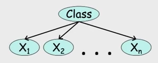
• The overall idea of NBM is, behind the data (represented by $x$), there is a variable denoting the “Class” (represented by $C$) upon which all variables depend. Once the class is determined, the variables are independent of each other. The joint probability distribution is $$p(C;x_1,x_2,...,x_n)=p(C)\Pi_{i=1}^n p(x_i|C)$$
• The Naive Bayes Model can be used as classifier (Naive Bayes Classifier). The algorithm is to find the MAP estimation of class: the class that maximizes $P(C|x_1, x_2, …)$.
• Practical note: In implementation, NBM uses a “add-one” rule, in order to avoid each of the probabilities to fall down to zero. Why? Usually when there is a zero probability, the reason is not that this class shall not contain this data, but because your training data is not large enough to include the data in this class.

Example: Bayesian Tracking, Temporal Model and Plate Model

• Another example of Bayesian estimation is Bayesian Tracking. The underlying idea is to update a posteriori estimation after each observation.
• Let us first look at the system. It can be represented by the following Bayesian Network:
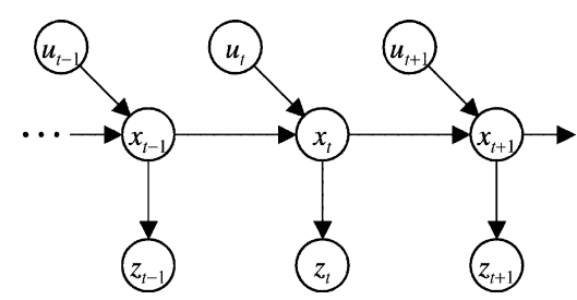
• where x is the state variable, y is the observation, u is control signal, v and w are two sources of random noises. z is observable whereas x and u are not. With the knowledge about the system state transition (a.k.a: $p(x_t|x_{t-1})$) and the measurement model (a.k.a: $p(z_t|x_t)$), you want to give an estimation about the state variable x at each time step.
• The algorithm is as following.
  First give a prior estimation (guess) about x: $p(x_0)$.
  Then for each time step:
  Calculate the a priori estimation: $$p(x_t|z_{1:t-1}) = \sum_{x_t} p(x_t|x_{t-1}) p(x_t|z_{1:t-1})$$ Calculate the a posteriori estimation: $$p(x_t|z_{1:t}) = p(x_t|z_t,z_{1:t-1}) = \frac{f(z_k|x_k,z_{1:k-1}) f(x_k|z_{1:k-1})}{f(z_k|z_{1:k-1})} = \frac{f(z_k|x_k) f(x_k|z_{1:k-1})}{Const}$$
• In the last line, the $z_{1:k-1}$ term is dropped.
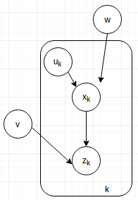
  Why? Because $z_k$ does not depend on $z_{1:k-1}$ since the previous state is given. Similarly, the denominator is just a normalization constant.
• The graphical model above is an example of temporal model, where many repetitive steps occur together. Hence a plate model can be used to simplify the graph.
• Sidenote: the PGM for Bayesian tracking without random noise is actually a Hidden Markov Model (HMM).

From Directed to Undirected Model

• Above mentioned are Bayesian Network. The other most common type of PGM, Markov Random Field, is represented by undirected graph models.
• Vertices still represent random variables, and edge represent the inference between the variables.
• We talk more about “infernce” instead of “dependency” in undirected models.
• The probability here is instead written as factor. For example, the MRF $x - y - z$ corresponds to the factor $\psi(x,y)\psi(y,z)$.
• Converting a directed model to an undirected graphical models loses some information. Also, moralization should be performed. The moralization process is needed when two or more nodes are parents of a child node. In order to keep the inference flowing, in MRF all parents should be connected (into a clique).
• An example shows the necessity of moralization. In a v-structured model ($x\rightarrow w \leftarrow y$), the probability is $p(x)p(y)p(w|x,y)$. However, without moralization, the factor representation of $x-w-y$ is $\psi(x,w)\psi(w,y)$. There should be a term considering w,x,y simultanuously but there is not! So x and y should be “moralized”.
• A clique in a MRF is a subgraph where every single nodes are connected to everyone else.

Exact Inference

• Problem: given a joint probability distribution $p(X_1, X_2, ...)$ (where $x_i, x_{i+1}...$ are unobserved), evaluate the marginaliation over unobserved variables.
• Naively marginalize over all unobserved variables require an exponential number of computations.
• Use Variable Elimination to compute marginalization. Push some variables inside.
• During elimination of each variable, an induced graph is produced.
• The width of an induced graph is number of nodes in the largest clique minus 1.
• Define the tree width (or minimal induced width) of a graph to be the minimum of the induced graph width (when eliminating according to a particular ordering).
• Finding the best elimination ordering (also computing the tree width) is NP-hard.

Message Passing and Belief Propagation

• Some information from this section is taken from CSC412 slides at University of Toronto, this tutorial and this note
• A message is a re-usable partial sum for the marginalization calculations.
• Message can be passeed from nodes to nodes. For example, the message from variable j to variable i (coming into the node $x_i$) is: $$m_{ji}(x_i)=\sum_{x_j}\psi_{ij}(x_i,x_j) \Pi_{k\in \eta (j) \backslash i} m_{kj}(x_j)$$ where $\eta(j)$ contains all neighbouring nodes of j.
• The marginal probability at a node is the produce of all incoming messages at that node: $$p_i (x_i)=\Pi_{j\in \eta(i)} m_{ji}x_i$$
• Sum-product Belief Propagation (root-to-leaf, and then leaf-to-root)
• Max-product BP
• Comparison of max product versus sum product.
• Loopy BP algorithm