This blog contains some notes about Automatic Speech Recognition (ASR), from earlier stage to some recent works. I try to plot a roadmap to have an idea of the big pictures out there.
- How human and computer process acoustic signals.
- The traditional GMM-HMM approach.
- The Connectionist Temporal Classification approach.
- The Sequence-to-Sequence approach.
Hearing the voice
First off, what is sound, or acoustic signals?
They are just fluctuations, which can be stored and read as a list of numbers. There are usually 16,000 numbers describing one second of sound, and we say the audio has a frame rate 16kHz.
How do we hear them?
It is via a mechanism in our ears, the eardrum. They fluctuate, driven by the energy, and convert the movements into bioelectrical signals. When these signals are passed to our brain, we hear sounds in different frequencies. Moreover, we are more sensitive to small frequency differences in the low frequency domains.
How about computers?
Computers process vectors, and algorithms are confused by too long sequences. It would be great if we can compress the one-dimensional, long sequence into shorter, multi-dimensional vectors which contain information. Besides, the information better relate to the energy contained in the waves. This is how Mel-scaled Frequency Cepstral Coefficients (MFCC) come in to the play.
MFCC characterize the sound waves with energy in different frequency domains (the so-called “Mel scaled frequency bins”), per time frame (usually 40ms). 40ms is usually long enough to give a good estimation about the energy (using either Fast Fourier Transform or Discrete Cosine Transform) in that frequency bin, and short enough to be precise, for speech signals that human can process.
What is the Mel scale then? It is approximately a transform from frequency (Hz) to the log scale: . Note that a change in lower frequency domain corresponds to a relatively larger change in Mel scale, than a high frequency one.
More details of calculation in MFCC can be found at this tutorial.
In practical, we can compute mfcc with off-the-shelf libraries, like pyAudioAnalysis and librosa. Usually we take 13 frequency bins, plus the base rate, and include their first- and second-order derivatives (“delta” and “delta-delta”), which add up to 42 dimensions.
Now that we have two-dimensional vectors of shape (length x 42). Automatic Speech Recognition systems take in these vectors and attempt to translate them into texts. This is a classic machine learning application, and I will briefly (arbitrarily) divide them into three avenues: GMM-HMM, CTC, and Seq2Seq.
The traditional GMM-HMM approach
Traditionally, ASR is a problem closely related to statistics. In each time frame (usually 40ms, or 25 ms, whatever) there is possibility that the speaker is talking about each phone (e.g., ‘ah’). There are 39 phones, and a Gaussian Mixture Model computes the probabilities of each phone in each time frame, given the frequency cepstral coefficients.
A temporal model (usually Hidden Markov Model; there are other options), is used to predict the word the speaker is talking about, given the phones. To make the predictions go with language syntaxes, a language model (usually N-gram) might be needed as well. Overall, the inference and training can resort to traditional HMM approaches, namely forward algorithm and viterbi algorithm.
Kaldi provides a lot of these models (“recipe”). Still state-of-the-art (as low as 3% word error rates) in a lot of speech recognition tasks, GMM-HMM approach do not require too many data (they could work well on small corpus containing as few as 10 hours of speech).
Side note 1: there are some bash and perl scripts in Kaldi, which could be an overhead for people new to ASR.
Side note 2: For more detailed descriptions for traditional GMM-HMM approaches see CSC401 slides here.
We basically need two models: an acoustic model that converts sound into phones, and a language model that combines phones to sentences. Each of these two models can be replaced with neural networks, which will be the main topics in following sections.
The Connectionist Temporal Classification approach
CTC was first proposed by Graves et al (ICML 2006). They use a recurrent neural network (RNN) as acoustic model. An RNN takes in a sequence of vector input, and give a prediction of character (instead of phone) every time step. There is a problem though: a speaker might say letter “C” for three frames, and then letter “A” for only one frame, then “T” for two frames. If classified correctly, the RNN outputs “CCCATT”. This should be treated the same as the case of “CCAT”, and “CAT”, and etc. There are actually many possibilities, as can be represented as paths in the decode graph.
Connectionist Temporal Classification considers the probabilities of all these possible paths as all outputting “CAT”, and sum them up to acquire the probability of the decoded path. The model optimizes the probability of all the paths constructing the correct text sequences.
There is another problem here: The word “TOO” could be classified as “TO”. CTC avoids this problem by introducing a “blank” letter (Note: this is different letter from the whitespace letter). The “blank” letter represents the border between letters. If we write “-“ as the blank letter, then “TO-O” and “TOOO-OO” will be regarded as “TOO”, while “TOOOO” will be regarded as “TO”.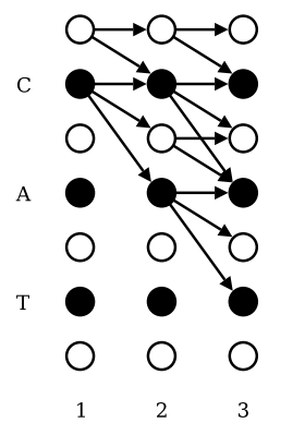
In practice, the RNN is usually a bidirectional LSTM. With CTC setting, you can take the advantage of the expressiveness of (recurrent) neural networks. Also, TensorFlow (probably as early as v1.0) and PyTorch (will support; starting from 0.5.0) implement optimized CTC loss, in which you can use conveniently.
In more recent years, some alternatives of RNN is also considered, and an impressive choice is Gated Convolution neural networks (GCNN).
GCNN (Dauphin et al, 2016) originates from Time-Delayed Neural Network (TDNN) (Waibel et al, 1989), which is also termed one-dimensional convolution. Note that the convolutional neural networks actually does a filtering operation (in the terms of the signal processing field). What’s different from CNN is that, a CNN layer basically performs a filter step:
where W (shape w x n) consists of n filters of width w, and the operator is linear filter.
Whereas a GCNN contains an additional gate:
where W and V are filters, and b and c are biases. means element-wise multiplications here. All filters and biases are trainable parameters.
Facebook Research used GCNN for speech recognition tasks. In additional to GCNN, they proposed a modification of CTC, which they term Auto Segmentation (ASG). Different from CTC, ASG discards the additional “blank letter”, and use the unnormalized graph loss terms instead. (The graph loss term is quite complicated, but luckily they open sourced their codes, via wav2letter). Recently, their improved work (Zeghidour et al, 2018) got very good results when learning from raw waveforms (by adding an additional layer to convert raw waveform into cepstral coefficients).
The Sequence to Sequence approach
Taking the automation idea one step further, we want to let neural networks take the place of complicated algorithms and let everything optimize on their own. Thus came the Seq2Seq network (Sutskever et al, 2014). They originally used this to do translation, but Seq2Seq can be applied to ASR directly (a.k.a: translation from speech to text). A RNN, “encoder”, compresses the input signal to a fixed length vector, and another RNN, “decoder”, finds the probability of the text character given previously decoded sequences and the compressed “context” vector. If a language model is incorporated, the score is added with one calculated by LM w.r.t the syntactic correctness.
As a sidenote, Viterbi decoding guarantees an optimal solution, but its complexity is where S is state space, which is lethal for word-based decoding. Beam search is usually used instead. In beam search decoding, instead of computing the possibilities of all paths, only those extending from a basket (size B) of best candidates in this step are considered. Then only B of these paths are preserved for the next decoding step.
Listen-Attend-Spell (Chan et al) is an application. Note that sequence to sequence learning requires humongous corpus of training data. Listen-attend-spell is trained on Google Voice Search with over 2000 hours (around 20 times the size of WSJ dataset).
As another sidenote, RNN-based Seq2Seq networks are starting to be replaced by Transformer (Vaswani et al, 2017). There are various forms of Transducers as ASR systems out there.
What’s next?
I think three approaches will be desirable for future developments of ASR systems.
The first path is via better engineering and stronger computational resource. Baidu’s DeepSpeech has great CTC implementations closely tied to the GPU cores. That allows training on large corpus.
The second path is paved with newer models that either allows machine to learn how to align automatically or gives machine easier paths to automatically back-propagate the useful knowledge.
The third path is more industry-aligned, which is context-dependent ASR models. Many groups of people speak hugely differently. Instead of training a model that suits all of them, it might be worthy to train several models for each of them. Some parameters could be shared.